Heuristic Capacitated Vehicle Routing Problem Solver • heumilkr

heumilkr provides an implementation of the Clarke-Wright algorithm (Clarke and Wright 1964) to find a quasi-optimal solution to the Capacitated Vehicle Routing Problem. It is available as an R package and as a Python package, which share the same C++ core.

Besides deliveries, it also supports “backhaul”: sites with negative demand have goods picked up and brought back to the depot, in any order within a run as long as the load stays within the vehicle capacity.

For a fixed number of vehicle types, the run time grows at best quadratically and at worst cubically with the number of sites $n$ . On the problems we tested with randomly placed sites and up to 4000 sites, it grew roughly like $n^{2}$ to $n^{2.1}$ , and roughly like $n^{3}$ if a limited vehicle type repeatedly runs out (see Runtime Benchmarks).

Installation

R

You can install the latest CRAN release of heumilkr with:

install.packages("heumilkr")

Alternatively, you can install the development version of heumilkr from GitHub with:

# install.packages("devtools")
devtools::install_github("lschneiderbauer/heumilkr")

Python

You can install the latest PyPI release of heumilkr with:

pip install heumilkr

Alternatively, you can install the development version of heumilkr from GitHub, which requires a C++ compiler, with:

pip install git+https://github.com/lschneiderbauer/heumilkr

The only dependency is NumPy. Install heumilkr[pandas] to also get pandas for Solution.to_pandas().

Example

R

The following example generates random demands at random locations, defines two vehicle types, applies the Clarke-Wright algorithm to generate quasi-optimal vehicle runs, and shows the resulting vehicle run solution.

library(heumilkr)
set.seed(42)

# generating random demand
demand <- runif(20, 5, 15)

# generating random site positions
positions <-
  data.frame(
    pos_x = c(0, runif(length(demand), -10, 10)),
    pos_y = c(0, runif(length(demand), -10, 10))
  )

solution <-
  clarke_wright(
    demand,
    dist(positions),
    # We have an infinite number of vehicles with capacity 33 available,
    # and two vehicles with capacity 44.
    data.frame(n = c(NA_integer_, 2L), caps = c(33, 44))
  )

print(solution)
#> $runs
#>   run vehicle max_load  distance
#> 1   0       0 25.78821 16.929475
#> 2   1       0 31.75943 29.029139
#> 3   2       1 34.12677 20.601801
#> 4   3       1 41.60558 30.176394
#> 5   4       0 22.65398 14.329082
#> 6   5       0 21.76854 14.231704
#> 7   6       0 14.34672  6.043174
#> 8   7       0 30.58007 36.895550
#> 
#> $sites
#>    site    demand
#> 1     0 14.148060
#> 2     1 14.370754
#> 3     2  7.861395
#> 4     3 13.304476
#> 5     4 11.417455
#> 6     5 10.190959
#> 7     6 12.365883
#> 8     7  6.346666
#> 9     8 11.569923
#> 10    9 12.050648
#> 11   10  9.577418
#> 12   11 12.191123
#> 13   12 14.346722
#> 14   13  7.554288
#> 15   14  9.622928
#> 16   15 14.400145
#> 17   16 14.782264
#> 18   17  6.174874
#> 19   18  9.749971
#> 20   19 10.603327
#> 
#> $visits
#>    run site order      load
#> 1    1    0     2  0.000000
#> 2    0    1     0 11.417455
#> 3    1    2     0 23.898031
#> 4    3    3     1 21.954433
#> 5    0    4     1  0.000000
#> 6    2    5     0 23.935806
#> 7    2    6     2  0.000000
#> 8    3    7     0 35.258910
#> 9    2    8     1 12.365883
#> 10   4    9     0 10.603327
#> 11   5   10     0 12.191123
#> 12   5   11     1  0.000000
#> 13   6   12     0  0.000000
#> 14   3   13     3  0.000000
#> 15   7   14     1  6.174874
#> 16   3   15     2  7.554288
#> 17   7   16     0 15.797802
#> 18   7   17     2  0.000000
#> 19   1   18     1 14.148060
#> 20   4   19     1  0.000000

# returns the total cost / distance
# (the quantity that is minimized by CVRP)
print(milkr_cost(solution))
#> [1] 168.2363

# returns the savings resulting from the heuristic optimization procedure
print(milkr_saving(solution))
#> [1] 168.7352

The R package has a built-in plotting function (using ggplot) for the result. The individual runs are distinguished by color. The site locations are marked with round circles while the depot is depicted as a square. The line types (solid/dashed/…) are associated to different vehicle types.

plot(solution)

Python

The following example solves a small problem with a fixed set of demands and distances, applies the Clarke-Wright algorithm to generate quasi-optimal vehicle runs, and shows the resulting vehicle run solution.

import heumilkr as hm

solution = hm.clarke_wright(
    demand=[3, 2, 4, 2],
    # distances between all locations, the first one is the depot
    distances=[
        [0, 1, 1, 2, 3],
        [1, 0, 2, 1, 2],
        [1, 2, 0, 3, 4],
        [2, 1, 3, 0, 1],
        [3, 2, 4, 1, 0],
    ],
    # one vehicle with capacity 6, and an unlimited number with capacity 9
    vehicles=[hm.Vehicle(capacity=6, count=1), hm.Vehicle(capacity=9)],
)

for run in solution.runs:
    print(run)
#> Run(id=0, vehicle=1, sites=(0, 2, 3), loads=(6.0, 2.0, 0.0), distance=6.0, max_load=9.0)
#> Run(id=1, vehicle=0, sites=(1,), loads=(0.0,), distance=2.0, max_load=2.0)

# returns the total cost / distance
# (the quantity that is minimized by CVRP)
print(solution.cost())
#> 8.0

# returns the savings resulting from the heuristic optimization procedure
print(solution.saving())
#> 6.0

How the Algorithm Works

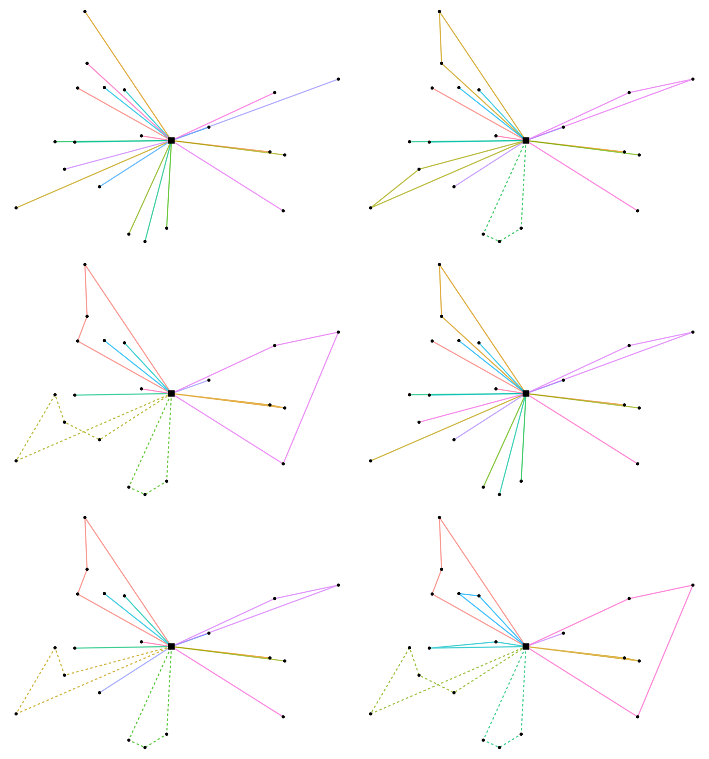
The following animation, made with the R package, shows how the Clarke-Wright algorithm iterates to arrive at its final solution:

Runtime Benchmarks

The benchmarks were taken on an Intel® Xeon® CPU E3-1231 v3 @ 3.40GHz CPU, through the R package using bench. The solver itself is the same C++ code in Python, but converting inputs and results adds some overhead that differs between the two packages.

The following graph shows the run time on one kind of problem: uniformly distributed random sites, demands between 5 and 15 and a vehicle capacity of 33. It amounts to $\sim 764µs$ for $n = 110$ , $\sim 26.9ms$ for $n = 1010$ , and $\sim 110ms$ for $n = 1910$ . Run times can differ for other problems.

Documentation

The two packages have separate documentation sites:

R package: website with the function reference and the articles.
Python package: API reference.

Feature Differences

Both packages include the solver with all its options (backhaul, vehicle types and restrictions) and calculate the cost and savings of a solution. The following is only part of the R package:

plotting a solution,
downloading and solving CVRPLIB instances,
the performance vignette, although its results also apply to the Python package, since they measure the shared solver.

References

Clarke, G., and J. W. Wright. 1964. “Scheduling of Vehicles from a Central Depot to a Number of Delivery Points.” Operations Research 12 (4): 568–81. https://doi.org/10.1287/opre.12.4.568.